ESTIMATION OF CONDUCTANCES 
  2 DIMENSIONAL CONDUCTANCE-BASED MODELS OF QUADRATIC TYPE

  This program estimates conductances in the subthreshold regime under
  the presence of subthreshold-activated ionic currents. The method is
  presented in C.Vich, A.Guillamon (2015), Journal of Computational
  Neuroscience.

  The estimation can be done in models that exhibit a parabolic nullcline 
  for the voltage and a linear nullcline for the recovery gating variable,
  i.e. the resonant currents (e.g slow potassium) and amplifying currents
  (e.g., persistent sodium).
  
  CELL TYPE: medial entorhinal cortex layer II stellate cells and CA1 
  pyramidal cells.


  Model needs to be quadratized (see Horacio G. Rotstein (2015) for more
  details about the quadratization procedure), that is, it has to be 
  written as:

       dv/dt = a*v^2 - w + Isyn(t) + Iapp
       dw/dt = eps*( alpha*v - lambda - w)
       
       such that 
           'v'      stands for the membrane potential.
           'w'      stands for the set of gating variables.
           'a'      controls the curvature of the v-nullcline.
           'alpha'  controls the slope of the w-nullcline.
           'eps'    stands for the time scale separation between v and w,
                    which tends to be small.
           'lambda' controls the relative displacement between the two
                    nullclines (the v one and the w one).
 
 
 
             ESTIMATION PROCEDURE - Required information

  We assume to have a quadratic approximation of a conductance-based neuron model, 
  as in H.Rotstein (2015). Given the resulting membrane potential (v) and 
  the course of the gating variable (w), this program estimates the synaptic 
  current that the neuron is receiving at each time. 
  Moreover, given the voltage traces for two different applied (steady) currents and the
  excitatory and inhibitory reversal potentials, the program estimates the excitatory and 
  inhibitory conductances separately.
  Finally, the program gives the option of estimating the synaptic
  conductance. This conductance can be estimated in two different ways: 
  (1)if only one voltage trace is given, the synaptic conductance
  is estimated using the synaptic reversal potential;
  (2) however, if two voltage traces are given (for two different applied currents), then
  the synaptic conductance can be either estimated using the synaptic reversal potential 
  or the leak conductance.
 
 
             INPUTS AND OUTPUTS

 * Input parameters:

   To run the program, write on the command window the next sentence 

           main_Estimation_Conductances(t,v,w,Iapplied)

   Such that:

         t: vector of length m containing the discretization of the time
            sample.

         v: m x n matrix containing n different samples of membrane
            potential corresponding at n different values of applied
            current.

         w: m x n matrix containing n different samples of the set of
            gating variables corresponding at n different values of applied
            current.

  Iapplied: vector of length n containing the different values of applied
            current. If its length is greater than or equal to 2, method
            discerns between the excitatory and the inhibitory conductances. 



 * Required parameters which are asked while running:

         a: parameter that controls the curvature of the v-nullcline.
     alpha: parameter that controls the slope of the w-nullcline.
    lambda: parameter that controls the relative displacement between the 
            two nullclines (the v one and the w one).
        vE: excitatory reversal potential (if the Iapplied vector has
            length greater than or equal to 2).
        vI: inhibitory reversal potential (if the Iapplied vector has
            length greater than or equal to 2).

   and, if you want to estimate the synaptic conductance,
   either
      vsyn: synaptic reversal potential.
   or
        gL: synaptic conductance (only if the Iapplied vector has
            length greater than or equal to 2).


 * Output parameters:

   The output parameters are given inside a .mat file called 'estimation.mat'
   such that

      Isyn: an m x n matrix containing the total synaptic current. Each
            column corresponds to a different value of applied current.

      gsyn: an m x n matrix containing the total synaptic conductance.
            Each column corresponds to a different value of applied
            current.

        gE: vector of length m containing the excitatory synaptic 
            conductance. It is only computed if, at least, 2 applied
            currents are considered.

        gI: vector of length m containing the inhibitory synaptic 
            conductance. It is only computed if, at least, 2 applied
            currents are considered.


 

             ADJOINT EXAMPLE presented in C.Vich and A.Guillamon (2015)

   A Matlab file called StellateModel.mat is added to the folder.
   This file contains all the needed inputs to simulate an estimation
   of the synaptic current, excitatory and inhibitory conductances and, giving the leak
   conductance, also estimate the synaptic conductances.
   Data comes from a reduced model for medial entorhinal cortex stellate cell 
   given in Rotstein et al (2006) that displays subthreshold oscillations. 
   The only considered activated currents in the model are the persistent sodium (INaP)  
   current and the h-(Ih) current.

   Detailed Usage (matlab command line excerpt):
>> load StellateModel.mat
>> [Isyn, gsyn, gE, gI]=main_Estimation_Conductances(t, v, w, Iapplied);
------ ESTIMATION OF CONDUCTANCES ------
Write the parameter that controls the curvature of the v-nullcline
a = 0.1
Write the parameter that controls the slope of the w-nullcline.
alpha = 0.4
Write the parameter that controls the relative displacement between the two nullclines
lambda = -.2
Estimating the synaptic current from v and w...
The synaptic current has been estimated.
Since the applied current vector has length greater than 1,
we are going to estimate the excitatory and inhibitory conductances
Write the excitatory reversal potential.
vE = 55
Write the inhibitory reversal potential.
vI = -25
Estimating the excitatory and inhibitory conductances...
Do you want to estimate the synaptic conductance? Yes (Y) or No (N)
gSyn estimation = 'Y'
Do you want to estimate the synaptic conductance using
the synaptic reversal potential (vsyn) or the constant leak conductance (gL)
option to estimate the synaptic conductance = 'gL'
Write the constant leak conductance
gL = 0.5
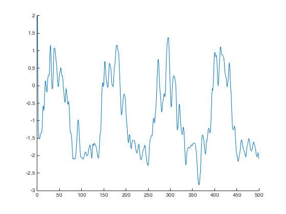
>> figure(); hold on; plot(t,Isyn(2,:),'-'); axis([0 500 -3 2]); hold off;
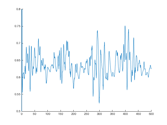
>> figure(); hold on; plot(t,gsyn,'-'); axis([0 500 0.5 0.8]); hold off;
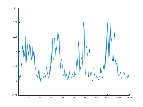
>> figure(); hold on; plot(t,gE,'-'); axis([0 500 -0.02 0.1]); hold off;
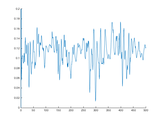
>> figure(); hold on; plot(t,gI,'-'); axis([0 500 0 0.2]); hold off;


These reproduce the dotted black traces in Figure 10A, 11A, 11B, 11C
respectively: