Example
An example walk-through is provided here to accustom you to the simulator. There are two windows to have opened for most simulations; a Terminal and a text editor or IDE.
- Open a Terminal and change the directory to the location of the simulator's mainDNF.py file.
- Open the values.py file in the same directory with a text editor or an IDE; preferably one that understands Python syntax because the interface is coded in Python.
Input
The input into the neural field from external sources, I, is on lines 80-83 of the
values.py file.
A baseline value of 2.0 is applied across the field and a 2D Gaussian curve is added before the initialization of I is complete.
On line 29 of the values.py file,
change the simulator view to visualize I by making the showData value equal to 3:
showData = 3Save the file and afterwards run the simulator by entering into the Terminal:
python mainDNF.py
A window similar to the image below will appear.
The window title shows the minimum and maximum values for I.
Most of the field has an input value of 2 and at the center is a sharp Gaussian curve raising the input to almost 10.
The view of I can be changed in ways expressed on the
Visualization page.

Press the Esc key on your keyboard to close the simulation window and exit the simulator.
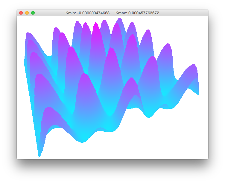
Kernel
The synaptic connectivity Kernel, K, is on lines 90-97 of the
values.py file.
These lines create a K that has spatial hexagonal connections.
K can be viewed in the simulator by changing the showData value to 4 on line 29 of the
values.py
file so that it reads:
showData = 4Save the file and then run the simulator again by entering into the Terminal:
python mainDNF.py
The simulator window (displayed below) shows the K field values and
the minimum and maximum values are written at the top.
K obeys periodic boundary conditions whereby K would appear continuous if copied and placed to every side of itself.
This can be seen by revolving the graph with a mouse.
Implementing other types of movement and different changes to the appearance of the graphed
K are shown on the Visualization page.
Press the Esc key on your keyboard to close the simulation window and exit the simulator.
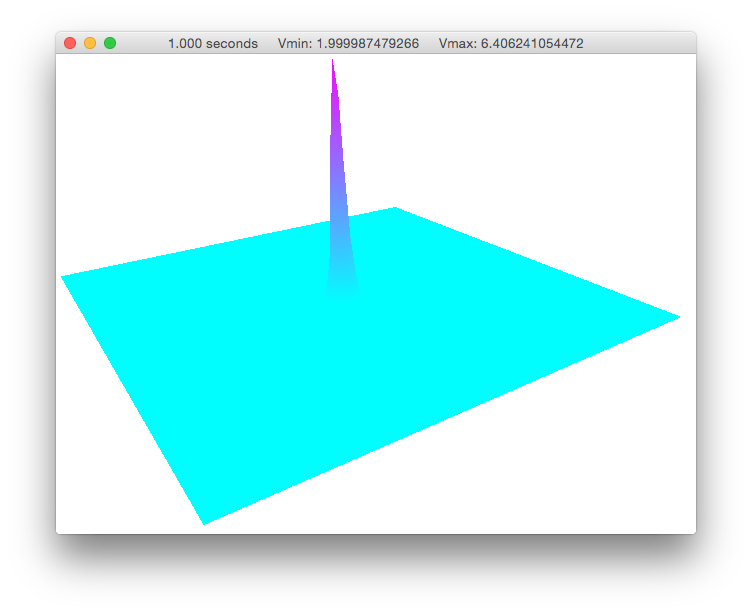
Voltage
The mean field voltage at the beginning of the simulation, V0, is initialized on line 60 of the
values.py file,
where it is set to 2.0 homogeneously across the field.
It can be changed to, for example, apply waves or noise to V0.
However, it will be kept as-is for the purpose of this example.
The simulator displays V over time when the showData value is set to 1 on line 29 of the
values.py
file so that it reads:
showData = 1Save the file and then run the simulator again by entering into the Terminal:
python mainDNF.py
Press the p button on your keyboard to begin the simulation in the window that appears.
The evolving V matrix is shown in the simulation of the equation
 .
.
The figure below shows a similar shape as I above.
This is because the K kernel matrix, also shown above,
consists of small fractions slightly above and below 0, moving the convolution of the integral close to 0.
I, with a maximum value near 10 at its center, is added to V's evolving shape.
Press the Esc key on your keyboard to close the simulation window and exit the simulator.
Propagation
V did not appear to spread from the large activity at the center of the
field in the figure above because K is very small.
Maximizing graph values around the flat surface of the graph will allow the activity spread to be seen.
To do this, run the simulator again by entering into the Terminal:
python mainDNF.py
Next, type: y
Then type and enter: 2.00007
As shown on the Visualization page, typing a number (2.00007 in this case),
preceded by y limits the maximum axis range to that number.
Type: p to begin the simulation, which will proceed similar to the figure below.
|
|
|
|


The field activity can be seen spreading at a very fast speed.
This is because the c value is large on line 43 of
the
values.py file.
When c≥l/√2Δt, the axon transmission speed is infinite and there is no transmission delay.
Press the Esc key on your keyboard to close the simulation window and exit the simulator.
Finite speed
Finite axonal transmission speed can be implemented on line 43 of the
values.py file by making
c<l/√2Δt.
Change c to 10 in the interface so that it reads:
c = 10 # mm/sSave the file and run the simulator again by entering into the Terminal:
python mainDNF.pyThe figure below shows the simulation with delayed activity spread over time. The effects of decelerated propagation speed are observed in the reduced field potential and also in the slower spread of activity when comparing the figures above and below.
|
|
|
|


