This is a multicompartmental Hodgkin-Huxley-type of model of a goldfish Mauthner cell. The building and usage of the model is
described in "Differential processing in modality-specific Mauthner cell dendrites" by Violeta Medan, Tuomo Maki-Marttunen,
Julieta Sztarker, and Thomas Preuss, Journal of Physiology (2017). The model is implemented in NEURON with Python interface.
Tuomo Maki-Marttunen, 2013-2017 (CC-BY 4.0).
Code files included:
I1.mod # A mod file for a sodium-type current
I2.mod # A mod file for a potassium-type current
mcell.hoc # An HOC file for running the simulations with square and ramp stimuli
mcell.py # A Python library for running the simulations, both one with square+ramp
# stimuli at soma and one with stimuli at the ends of dendrites. For an
# example on how to use the library, see runfit.py (the only script
# where this library is used)
mcell_activedend_varycoeffsL.py # A Python library for simulations with active dendrites
mcell_activedend_varycoeffs_activeL.py # A Python library for simulations with active ventral dendrite
minimizedimbydim.py # A Python library for minimizing a function dimension by dimension
mosinit.hoc # An HOC file that runs mcell.hoc
mytools.py # General Python tools
neurmorph.hoc # The neuron model initialization file
neurmorph_activedend.hoc # The neuron model initialization file, including active dendrites
runfit.py # A Python script for optimizing the neuron model parameters
runmauthner.py # A Python script for running simulations for Figure 7B
runmauthner_activedend_decays_varycond.py # A Python script for running simulations for Figure 9A
runmauthner_activedend_decays_varycond_activeL.py # A Python script for running simulations for Figure 9A
Data files included:
experimental_data.mat # A MATLAB file with experimental data with square and ramp stimuli
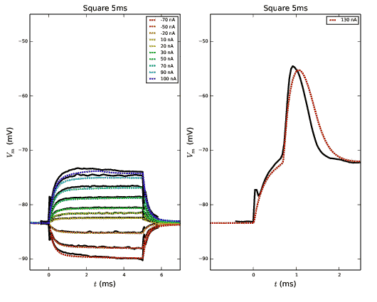
fit.eps # Figure 7B. Saved by runmauthner.py
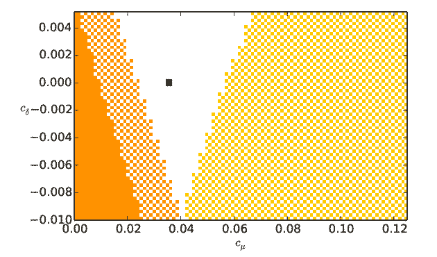
decay_orders_robustness.eps # Figure 9A. Saved by runmauthner_activedend_decays.py.
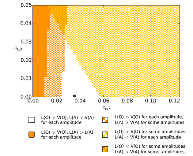
decay_orders_robustness_activeL.eps # Figure 9B. Saved by runmauthner_activedend_decays_varycond.py.
Data files saved by the scripts:
run*.dat # Data produced by mcell.hoc. Not used in this entry, however, as mcell.hoc is run
# from the Python interface (in runmauther.py) and the data is thus saved in the memory.
activedend_decays_varyconds.sav # Data for Figure 9A. Saved by runmauthner_activedend_decays.py. Used only if the
# script is run for a second time.
activedend_decays_varyconds_activeL.sav # Data for Figure 9B. Saved by runmauthner_activedend_decays_activeL.py. Used only if the
# script is run for a second time.
Before running the simulations, compile the mod files by typing
nrnivmodl
For simulating the model and plotting the results (in Python), run
python runmauthner.py
python runmauthner_activedend_decays_varycond.py
python runmauthner_activedend_decays_varycond_activeL.py
Output from runmauthner.py:
 Output from runmauthner_activedend_decays_varycond.py:
 Output from runmauthner_activedend_decays_varycond_activeL.py:
 The second and third simulations are relatively heavy (take approximately half an hour on a standard computer),
and once finished, the results are saved in activedend_decays_varyconds.sav and activedend_decays_varyconds_activeL.sav
for possible later use.
Alternatively, the model can be run with the HOC interpreter as follows
nrniv mcell.hoc
The second and third simulations are relatively heavy (take approximately half an hour on a standard computer),
and once finished, the results are saved in activedend_decays_varyconds.sav and activedend_decays_varyconds_activeL.sav
for possible later use.
Alternatively, the model can be run with the HOC interpreter as follows
nrniv mcell.hoc